The following table develops progressively more sophisticated
uses of Maxima as a symbolic math tool. Remember, you do not need to use or memorize
all of this table at once - simply go up to the point that your current needs
dictate, and return to this table when they become more extensive.
Note: in the third column some expressions have been typeset for greater ease
of reading.
| Topic |
Discussion |
Maxima Input |
Maxima Output |
| Basic typing |
Remember, use a semicolon and the enter key to terminate input. |
(2+5/6-sqrt(4))^2; |
25
--
36 |
| Using the previous line |
The % symbol tells Maxima to use the result of the previous calculation. |
%+1; |
61
--
36 |
| Using a line by name |
Alternatively, you can refer to a result you wish to use
by the name of its output line. |
D2+1; |
97
--
36 |
| Numeric evaluation |
To tell Maxima to calculate a floating point result, use the float function. |
float(%); |
2.694444444444445 |
| Defining a function |
To define a function: give it a name, followed by its independent variable
in parentheses, followed by the symbols :=, followed by its definition. |
f1(x):=x^2-5*x+6; |
2
f1(x) := x - 5 x + 6 |
| Using a function |
Once defined, you can use a function in an intuitive way. |
f1(5); |
6 |
| Assigning a value to a variable |
The : sign assigns a value to a variable. |
a:5; |
5 |
| The variable assignment will now be used everywhere in place of the variable
name. |
f1(a); |
6 |
| Defining an equation |
The = sign defines an equation. |
x=1-b*y; |
x = 1 - b y |
| Solving an equation |
An equation can be readily solved for any of its variables, if a simple
expression exists. |
solve(%,y); |
x
- 1
[y = - -----]
b |
| Another example, yielding both roots of a quadratic. |
solve(x^2+2*x-3=0,x); |
[x = - 3, x = 1] |
| In order to use any of the results from a solve step,
we need to "extract" them from the output list. |
%[2]; |
x = 1 |
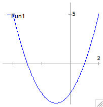
| Plotting a function |
Let's look at a plot of our function and see that the roots tally. The
second argument used by the plot2d function is a list, and is indicated
by square brackets ([]). This
particular
list specifies the x-range of interest. |
plot2d(x^2+2*x-3=0,[x,-4,2]); |
 |
| Systems of equations |
Maxima can also solve systems of equations, if the equations
and variables of interest are presented to it as lists. |
solve([x+3*y=3,2*x+5*y=5],[x,y]); |
[[x = 0, y = 1]] |
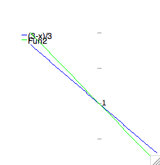
| Plotting multiple functions |
To plot multiple functions, we use a list of their names as the first
argument in the plot2d function. Let's use this feature to check the previous
result. |
plot2d([(3-x)/3,(5-2*x)/5],[x,-1,1]); |
 |
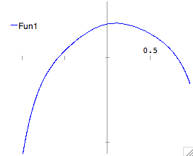
| Solving equations numerically |
Even when an analytic solution cannot be found, Maxima can in many cases
solve the equation numerically. Let's first examine this seventh-order
polynomial by plotting it. |
plot2d(x^7-5*x^6+4*x^4-5*x^2+x+2,[x,-1,1]); |
 |
| We see two roots between -1 and 1. To get their exact values, we load
the newton routine, and use it with a guess to the right of the root we
wish to get. |
load("newton");
|
/sw/share/maxima/5.9.0rc3/share/numeric/newton.mac |
| newton(x^7-5*x^6+4*x^4-5*x^2+x+2,1); |
8.194213634964119B-1 |
| We repeat the process for the second root. |
newton(x^7-5*x^6+4*x^4-5*x^2+x+2,0); |
- 5.763042928902195B-1 |
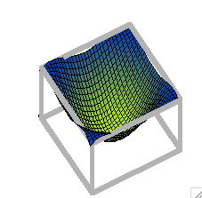
| Functions of multiple variables |
Multivariate functions are defined as before, but separating variables
with commas in the definition. |
f2(x,y):=sin(x^2+y^2);
|
2 2
f2(x, y) := SIN(x + y )
|
| f2(1,4); |
SIN(17)
|
| float(%); |
- .9613974918795568
|
| 3D Plots |
These are created as before, but using the plot3d command, and with separate
lists for the ranges of the x and y axes. |
plot3d(f2(x,y),[x,-1,1],[y,-1,1]); |
 |
| Factoring Polynomials |
Maxima can factor some polynomials. |
factor(x^2+2*x+1); |
2
(x + 1) |
| Expanding Polynomials |
Or expand them |
expand(%); |
2
x + 2 x + 1 |
| Simplifying Trigonometric expressions |
Much the same can be accomplished for trigonometric expressions. |
trigsimp(sin(x)^2+cos(x)^2); |
1 |
| Expanding Trigonometric expressions |
As with their expansion. |
trigexpand(cos(x+3*y));
|

|
| trigexpand(%); |
 |
| expand(%); |
 |
| Simplifying rational expressions |
In many cases, Maxima can simplify rational expressions |
fullratsimp((x^2+2*x+1)/(x+1)+1/(4*x+3)); |
 |
| Expanding rational expressions |
Or expand them. |
ratexpand((x^2-1)/(x+2)); |
 |
| Substituting the Results of One Calculation Into Another |
We can save ourselves quite a bit of typing by using substitutions. First,
we isolate the result we wish to substitute. |
solve(x^2-1=0,x);
|
[x = - 1, x = 1]
|
| %[2]; |
x = 1 |
| Then, we perform our substitution |
subst(%,y=3*x-11); |
y = - 8 |
| Calculating limits |
Let's create an interesting function, and calculate its limit as x approaches
0 |
f3(x):=sin(x)/x;
|
SIN(x)
f3(x) := ------
x
|
| limit(f3(x),x,0); |
1 |
| To calculate the limit from above, we simply add PLUS (or MINUS from
below) to our entry. |
limit(tan(x),x,%PI/2,PLUS);
|
MINF
|
| limit(tan(x),x,%PI/2,MINUS); |
INF |
| Simple Differentiation |
We can differentiate any function with respect to a given variable |
diff(c*x^2-sin(d*x),x); |
2 c x - d COS(d x) |
| Higher Order Differentiation |
Higher order differentiation is also readily available. |
diff(x^3,x,3); |
6 |
| Simple Integration |
We can also perform indefinite integration on a function (assuming a
simple closed form for the answer exists and is computable by Maxima). |
integrate(cos(3*x),x); |
SIN(3 x)
--------
3 |
| Definite Integration |
Or definite integration, if we enumerate the lower and upper limit. |
integrate(cos(3*x),x,0,%PI/2); |
1
- -
3 |
| Numeric Integration |
In cases where a closed form integral is unavailable, Maxima can compute
the result numerically. |
integrate(sin(sin(x)),x,0,1);
|
 |
| romberg(sin(sin(x)),x,0,1); |
.4306059236425572 |
| Summation |
Summations can be written out. |
sum(1/(n^2),n,1,INF); |
 |
| If desired, they can be evaluated by setting SIMPSUM to TRUE. |
SIMPSUM:TRUE;
|
TRUE
|
| sum(1/(n^2),n,1,INF); |
2
%PI
----
6 |
| Products |
Products work in much the same way. |
product(1/(n^2),n,1,10); |
1
--------------
13168189440000 |
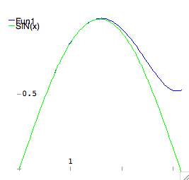
| Series Expansion |
Series expansions can also be computed. Let's calculate the series
expansion of the sine function around x=0, up to the fifth power in x. |
taylor(sin(x),x,0,5); |
3 5
x x
/T/ x - -- + --- + . . .
6 120 |
| Since the output of taylor has special properties, we need to convert
it into a polynomial. |
trunc(%); |
3 5
x x
x - -- + --- + . . .
6 120 |
| We can now compare our series approximation to the original function. |
plot2d([%,sin(x)],[x,0,%PI]); |
 |
We welcome your feedback on this workflow/tutorial - please email us at symmath@hippasus.com
